Backpropagation in 60 Seconds (Interview-Ready, No Fluff)

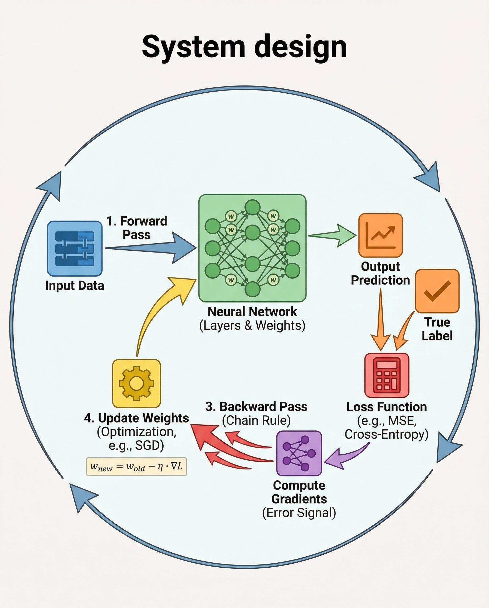
Backpropagation is how neural networks learn: it computes the gradient of the loss with respect to every weight using the chain rule. Below is a compact, interview-ready walkthrough you can state and derive on the spot.

1) Forward pass

• Run inputs through each layer to get predictions.
• Compute the scalar loss L(prediction, target).

2) Backward pass (chain rule in action)

• Start at the output and propagate error backward, layer by layer, using activation derivatives.
• For a weight w that affects output y: ∂L/∂w = ∂L/∂y * ∂y/∂w. That local multiplication of sensitivities is the chain rule.
• Common layer formula (vector form):
  • δ^L = ∂L/∂a^L * σ'(z^L) (output error)
  • For l = L−1..1: δ^l = (W^{l+1}^T δ^{l+1}) * σ'(z^l)
  • Gradient for weights: ∂L/∂W^l = δ^l (a^{l-1})^T

3) Update

• Move weights opposite the gradient (gradient descent):

  w ← w − η ∇L

Quick pseudocode

# Forward
for l in 1..L:
  z[l] = W[l] @ a[l-1] + b[l]
  a[l] = σ(z[l])
loss = Loss(a[L], y)

# Backward
δ[L] = dLoss/da[L] * σ'(z[L])
for l in L-1..1:
  δ[l] = (W[l+1].T @ δ[l+1]) * σ'(z[l])
  dW[l] = δ[l] @ a[l-1].T

# Update
for l in 1..L:
  W[l] -= η * dW[l]
  b[l] -= η * db[l]

Why this matters (short intuition)

• Efficiency: backprop computes all partial derivatives in time proportional to a few times a forward pass (not one pass per weight).
• Scalability: it makes training deep networks practical by reusing intermediate computations (activations and local derivatives).

Common interview talking points

• Explain the chain rule and derive ∂L/∂w for a single neuron.
• Show how gradients flow from output to input using the δ recurrence.
• Mention practical issues: vanishing/exploding gradients (sigmoid vs ReLU), and how initialization, normalization, and skip connections help.
• Contrast with numerical gradients (finite differences) and note autodiff does this efficiently and exactly (up to floating point).

Remember: keep the derivation clear, show one example neuron, and state the update rule. That's concise, correct, and interview-ready.

#MachineLearning #DeepLearning #AI